

CORRELATIONS & CAUSAL ANALYSIS
METHODS AND EXCEL ANALYZERS
Learn, download the Excel templates, practice and check your skills

13 Correlations & Scatter Plots
14 Hypothesis Testing with t-Test

15 Analysis of Variance (ANOVA)
16 Randomized Experiments

17 Exploratory Causal Analysis
13 Correlations & Scatter Plots
1. Learn
PERFORMANCE OBJECTIVES
At the end of this module, you will know how to:
- Conduct a bi-variate correlation analysis and visualize the results with a Scatter Plot;;
- Calculate and interpret the Pearson's Correlation factor.
This module includes opportunities to practice and assess your skills to conduct this type of analysis.
ABOUT CORRELATIONS AND SCATTER PLOTS
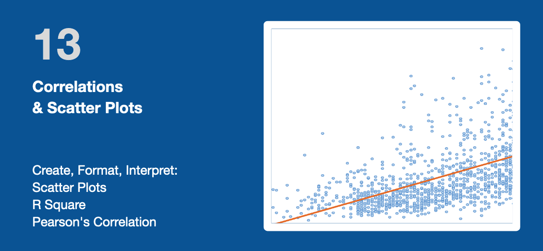
Correlations & Scatter Plots help analyze the "degree of relationship" between two variables: a so-called bi-variate analysis. Correlation is typically expressed as a Correlation Factor r ranging from -1 to +1:
- Positive values of correlation indicate that as one variable increase the other variable increases as well.
- Negative values of correlation indicate that as one variable increases the other variable decreases.
The most commonly used type of correlation is Pearson correlation. It is named after Karl Pearson, who introduced this statistic around the turn of the 20th century. Pearson's r measures the linear relationship between two variables, say X and Y.
- A correlation of 1 indicates the data points perfectly lie on a line for which Y increases as X increases.
- A value of -1 also implies the data points lie on a line; however, Y decreases as X increases.
A Scatter Plot is a graph to visualize the relationship between two variables or sets of data.
Note: the Pearson's Correlation factor was developed by Karl Pearson, English mathematician and biostatistician from an idea originally introduced by Francis Galton in the 1880s.
SKILL PRACTICE
1. Download the attached XLS file:
- The first tab contains Sample Data;
- The second tab Scatter Plots & Correlations explains the steps to create a Scatter Plot and estimate the correlation factor;
Please practice your skills in the tab Skill Practice: first, an easy practice then a more difficult practice.
2. Report the outcome of your practice in the Skill Assessment quiz.
2. Download & Practice
3. Check Your Skills
Refresh the page to retake the test or explore additional member resources
14 Hypothesis Testing with t-Test
1. Learn
PERFORMANCE OBJECTIVES
At the end of this module, you will know how to:
- Conduct and interpret a 2-Sample t-Test Assuming Unequal Variances;
- Conduct and interpret Paired Sample t-Test.
This module includes opportunities to practice and assess your skills to conduct this type of analysis.
WHAT IS A t-TEST?
Significance or Hypothesis Testing evaluates the plausibility of two hypotheses so that only one can be right. There are many statistical tools and methodologies to conduct this type of analysis. In this module, we will describe and practice how to conduct the following two types:
- 2-sample t-test assuming unequal variances: for instance, this analysis can be used to compare the performance of learners before versus after an intervention; or analyze the difference of two groups in a randomized A/B Testing experiment;
- Paired sample t-test: in this type of analysis, each subject or learner is measured twice, resulting in pairs of observations. This can be used to measure the effectiveness of a training courses for the same class of learners, by comparing their pre-test versus post-test scores. Note: t-test is best used when the sample size is small (n<100) and the population variance is unknown. For much larger sample size or the population variance is known, it is recommended to use Z-test.
Hypothesis Testing starts by stating two hypotheses so that only one can be right. In the above example, the hypothesis could be formulated as:
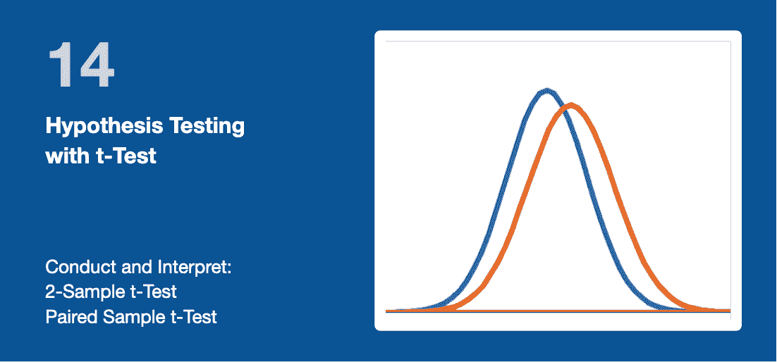
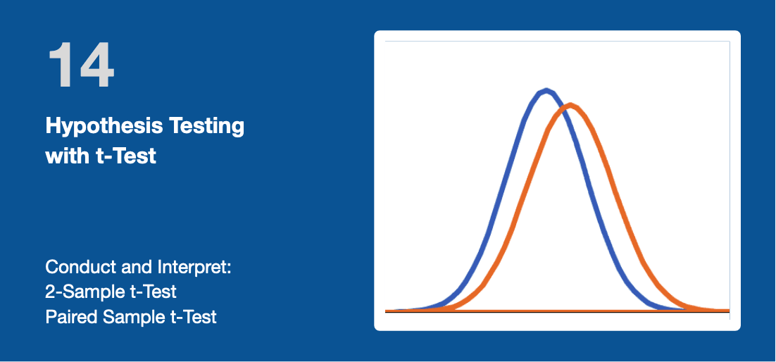
- There is no difference in performance before and after the intervention. Or, there is no difference between the learners' pre-test and post-test scores. We call this hypothesis the Null-Hypothesis or H0.. In the graphic below, the two distribution curves overlap;
- There is a statistically-significant difference between the two dataset. This is the Alternative Hypothesis or Ha (sometimes referred as H1).
Hypothesis Testing works best when you compare two datasets with a normal distribution. In some cases, the two datasets might appear to be different because their mean or standard deviation values are different. By taking account all data in the dataset, Hypothesis Testing provides the statistical evidence that two dataset are significantly different or not.
Not finding enough evidence to reject the null hypothesis does not imply that the dataset are equal, just that there was not enough evidence to conclude that they are different. There are many potential reasons why the Null-Hypothesis can not be rejected: the most common one is that the sample size was too small to provide sufficient evidence.
Is the difference significant?
Note: The first known hypothesis test was the Trial of the Pyx, a periodic ritual of the Royal Mint in London. This started in 1279. Each time the Mint made coins, a small number of them went into the Pyx, a wooden box. When a Trial was convened, independent goldsmiths compared the selected Pyx coins to standards in order to validate that newly produced coins were within prescribed tolerances for weight and composition.
SKILL PRACTICE
1. Download the attached XLS file:
- The first tab contains Sample Data;
- The second tab Hypothesis Testing explains the steps to conduct the two types of Analysis Testing;
Please practice your skills in the tab Skill Practice;
2. Report the outcome of your practice in the Skill Assessment quiz.
2. Download & Practice
3. Check Your Skills
Refresh the page to retake the test or explore additional member resources
15 Analysis of Variance (ANOVA)
1. Learn
PERFORMANCE OBJECTIVES
At the end of this module, you will know how to:
- Conduct and interpret a Single Factor ANOVA Analysis;
- Conduct and interpret a Two-Way ANOVA Analysis.
This module includes opportunities to practice and assess your skills to conduct this type of analysis.
WHAT IS ANOVA? HOW TO USE IT?
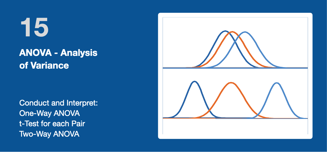
Analysis of Variance (ANOVA) is a statistical technique that is used to check if the means of two or more groups are significantly different from each other. ANOVA checks the impact of one or more factors by comparing the means of more than two datasets.
t-test hypothesis testing described in the previous module is a method that determines whether two groups are statistically different from each other. In contrast, ANOVA determines whether three or more populations are statistically different from each other. For instance, employees can be split into 3 or more groups by their level of experience, by department or by location. In addition, ANOVA allows to study the influence of multiple factors:
- A one-way ANOVA involves one factor or independent variable: like the influence of Performance Improvement intervention on 3 groups of employees;
- A two-way ANOVA examines the effect of two independent factors on a dependent variable. For instance, analyzing the test score of a class based on gender and age. The test score is a dependent variable; gender and age are the independent variables. ANOVA can be used to eliminate the need for pairwise comparisons, whenever they are not significant.
Note: ANOVA is also called the Fisher analysis of variance. The term became well-known in 1925, after appearing in Fisher's book, "Statistical Methods for Research Workers". It was later employed in experimental psychology and expanded to more complex subjects.
SKILL PRACTICE
1. Download the attached XLS file:
- The first tab contains Sample Data;
- The second tab Analysis of Variance (ANOVA) explains the steps to conduct an ANOVA analysis;
Please practice your skills in the tab Skill Practice: first, an easy practice then a more difficult practice.
2. Report the outcome of your practice in the Skill Assessment quiz.
2. Download & Practice
3. Check Your Skills
Refresh the page to retake the test or explore additional member resources

16 Randomized Experiments
1. Learn
PERFORMANCE OBJECTIVES
At the end of this module, you will know how to:
- Demonstrate causality by conducting a Randomized Experiment;
- Check three criteria to validate that a study is properly conducted as a Randomized Experiment.
This module includes opportunities to practice and assess your skills to evaluate Random Groups.
HOW TO CONDUCT A CAUSAL ANALYSIS WITH RANDOMIZED EXPERIMENTS?
Causal Analysis is about proving the relationship between the cause and its effects. For instance, does the new approach really make a difference? Are certified employees performing better than those who are not certified?
There are two techniques to analyze causation:
- Randomized Experiments (this module)
- Exploratory Causal Analysis (next module)
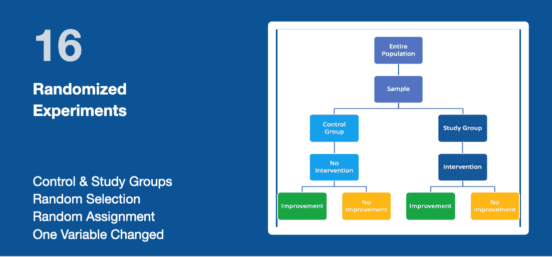
A Randomized Experiment is the most robust method for demonstrating a causal link between a cause and its effect. The approach is to define two random groups that are statistically equivalent. This minimizes the bias by balancing out individual characteristics between groups. These so-called confounding variables could otherwise impact the outcome.
For instance, select two populations of learners with a similar distribution of age, location, gender, job levels, performance level, conditions, etc... The only difference between the two groups is when the study group receives the intervention or treatment or new solution, while the control group will either get a placebo or continue their work without intervention.
A/B testing is a way to compare two versions of a single variable, typically by testing a subject's response to variant A against variant B, and determining which of the two variants is more effective. It is commonly used for:
- Email marketing to design the most effective web page or campaign;
- Product Pricing to determine the right price that will maximize revenue;
- Political campaigns to test and find out what voters are willing to support.
Note: if you can not deal with the entire population and work only with samples with both groups, then the samples you select should also be randomized. In summary, use the following three key criteria to design a Randomized Experiment:
- There is a Control group and a Study (or Experimental) group. Both groups have similar sizes;
- Participants are randomly selected from the overall population and randomly assigned to each group;
- Only one variable is changed between the two groups (going through the training program).
Note: Randomized experiments were popularized by C. S. Pierce in psychology and education in the late eighteen-hundreds. Outside of psychology and education, R.A. Fisher introduced additional principles of experimental design in his book Statistical Methods for Research Workers (source Wikipedia).
The first reported clinical trial was conducted in 1747 by James Lind, a Scottish doctor, responsible for the naval hygiene and treatment for scurvy in the british Royal Navy. Randomized experiments later appeared in psychology, where they were introduced by Charles Sanders Peirce and Joseph Jastrow in the 1880s.
SKILL PRACTICE
1. Download the attached XLS file:
- The first tab contains Sample Data;
- The second tab Random Groups explains the steps to check that your control and study groups are randomized;
Please practice your skills in the tab Skill Practice.
2. Report the outcome of your practice in the Skill Assessment quiz.
2. Download & Practice
3. Check Your Skills
Refresh the page to retake the test or explore additional member resources
17 Exploratory Causal Analysis
1. Learn
PERFORMANCE OBJECTIVES
At the end of this module, you will know how to:
- Apply a four step process to determining the plausibility of a cause-to-effect relationship;
- Visualize the Causal Chain of Evidence.
This module includes opportunities to practice the four steps and assess your skills.
WHAT IS AN ECA?
A study with randomized experiment as described in the previous module is the best way to demonstrate causality. Unfortunately, we do not always control the research or the way data are collected. In this case, an Exploratory Causal Analysis (ECA) offers an alternative approach to analyze causality. Grounded in statistical analysis and causal inference, this exploratory research replaces or precedes more formal causal research such as Randomized Experiments. It takes place in four steps:
- Demonstrate first that there is an association or correlation between the independent and dependent variable.
A robust correlation has a Pearson correlation factor greater than 0.7 (Refer to the module "Scatter Plots & Correlations"). Over time, you can also check for "Dose-Response" Relationship: your case for causality is stronger when there is a linear relationship between the size of the intervention (like the proportion of employees certified) and the effect (overall performance improvement). If you notice some difference between and after the intervention, you can perform a t-test or ANOVA to make sure that the difference is significant, and not only the results of random changes (check the respective modules). - Determining the time order of the variables
Obviously, the cause must precede the effect. For instance, if you compare the evolution of two groups (one receiving the intervention, the other not), then the effect should start taking place after the intervention. Check the module "Time-Series Analysis" for graphical representations; - Rule out alternative explanations
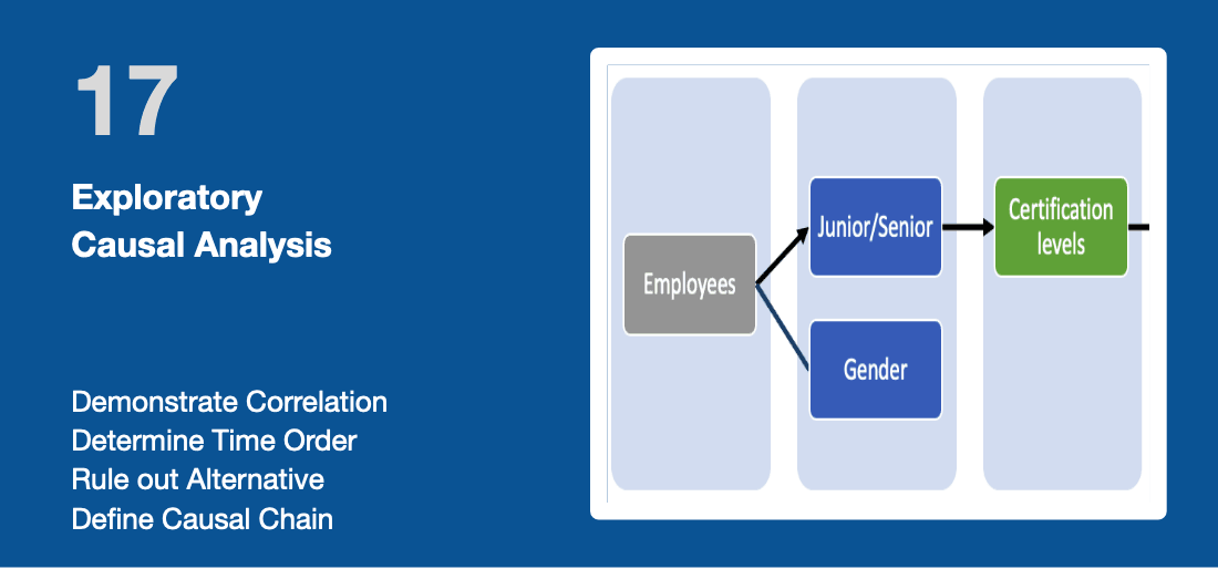
This is oftentimes the most difficult step to perform as it is easy to miss out confounding variables that have an effect on the outcome. This could lead to a False Positive (also called spurious correlation) i.e. a situation where we believe that causality exists when it does not. Finding a confounding variable is not the end of the analysis: in the contrary, this could lead to an additional cause or even to the root-cause of the change. You can use models like the 5 why’s or Ishikawa to perform a root-cause analysis. - Define the Causal Chain of Evidence
This is about determining the plausibility of the cause-to-effect relationship. The causal chain of evidence documents the step-by-step relationship between an intervention and its intended outcomes. In the field of Human Performance, the typical steps are.
- Training, job aids results, incentives influences our work behaviors. We become better at what we do;
- As a result, our individual performance measured by our work output improves;
- This leads to an improvement in the organization's performance (or business results) as the collective output of all employees.
Note: Aristotle already describes in 300 BC the four causes as elements of an influential principle. He classified explanations of change or movement into four fundamental types of answer to the question "why?". Aristotle wrote that "we do not have knowledge of a thing until we have grasped its why, that is to say, its cause."
SKILL PRACTICE
1. Download the attached XLS file:
- The first tab contains Sample Data;
- The second tab Exploratory Causal Analysis describes an example with sample data.;
Please practice your skills in the tab Skill Practice: first, an easy practice then a more difficult practice.
2. Report the outcome of your practice in the Skill Assessment quiz.
2. Download & Practice
3. Check Your Skills
Refresh the page to retake the test or explore additional member resources


